Electron Beam Track on Substrate

Goal

Simulation of a single track made by electron beam. Track geometry is studied: width, depth, height. The track shape is expected to be stable.

The material of the plate is Ti6Al4V.

Run

Copy the JSON file provided with the usercase into the simulation folder.

> cp <path>/EBP_track_plate.json .

Run the code from terminal with the provided JSON file. You may need to edit the information on the license file in it.

> INPUT_JSON_FILE=EBM_track_plate.json /opt/KiSSAM/start_calc.sh

Make sure that simulation is started by making sure there are no fatal errors in the .log file that has appeared. It might be necessary to insert the correct license filepath.

Input Configuration

The simulation parameters can be adjusted by editing the JSON file.

{
  "licenseFile": "/licences/kissam-end-2023-6-30.lic",
    "config": {
      "MaxTimesteps"         : 120000,
      "IterationSubstepsRate": 1000,
      "DumpDataRate"         : 12000,
      "AutoTermination": true,
      "DumpVTK"              : false,
      "DumpARR"              : false,
      "DumpVDB"              : true
    },
    "sizes": {
      "FullXapprox": 0.020
    },
    "Substrate": {
      "preheating"  : 293.0,
      "wettingAngle": 10
    },
    "Camera": {
      "AmbientGas": "Ar",
      "pressure"    : 0.4,
      "temperature" : 293.0
    },
    "Material": "Ti6Al4V",

    "ScanStrategy": {
      "Type": "SingleTrack",
      "SingleTrack": {
        "length"   : 10e-3,
        "startPosX": 5e-3,
        "startPosY": 4e-3
      },
      "Beam": {
        "type"     : "Ebeam",
        "Shape"    : "Gauss",
        "Power"    : 900.0,
        "Width"    : 500e-6,
        "Speed"    : 3.0,
        "ElectronsEnergy" : 60e3,
        "SuppressBackScattering": 0
      }
    },
    "MaterialsLibrary": {
      "Ti6Al4V": {
        "components"             : null
      }
    }
}

The parameters that are not specified here are taken from the /opt/KiSSAM/default.json file. Here we turned off the output of vtk files which contain temperature distribution and arr files to save on the storage taken by the simulation output. The config.Autotermination option is used to terminate the calculation when the beam reaches the end of the scanning path. For the EBM simulation, the ambient gas and pressure are specified. KiSSAM features multi-component evaporation model. The concentration of Ti and Al is not studied in this user case, therefore, we change the Ti6Al4V material properties to turn off the simulation of components distribution.

Simulation Results

The simulation runs for ~5 hours. The default name for the simulation output directory is output.

3D view

The track geometry is stored in the openVDB format output/geometry.vdb. It is updated during the simulation process and stores the latest state. View it with Blender or VDB view.

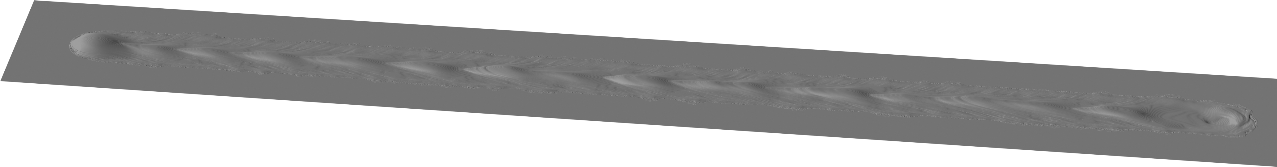
Fig. 25 openVDB file loaded and rendered in Blender

Images and animation output

The meltpool states are rendered as images and stored in output/rendered3D. The images of cross-sections are found in output/cross-sections.

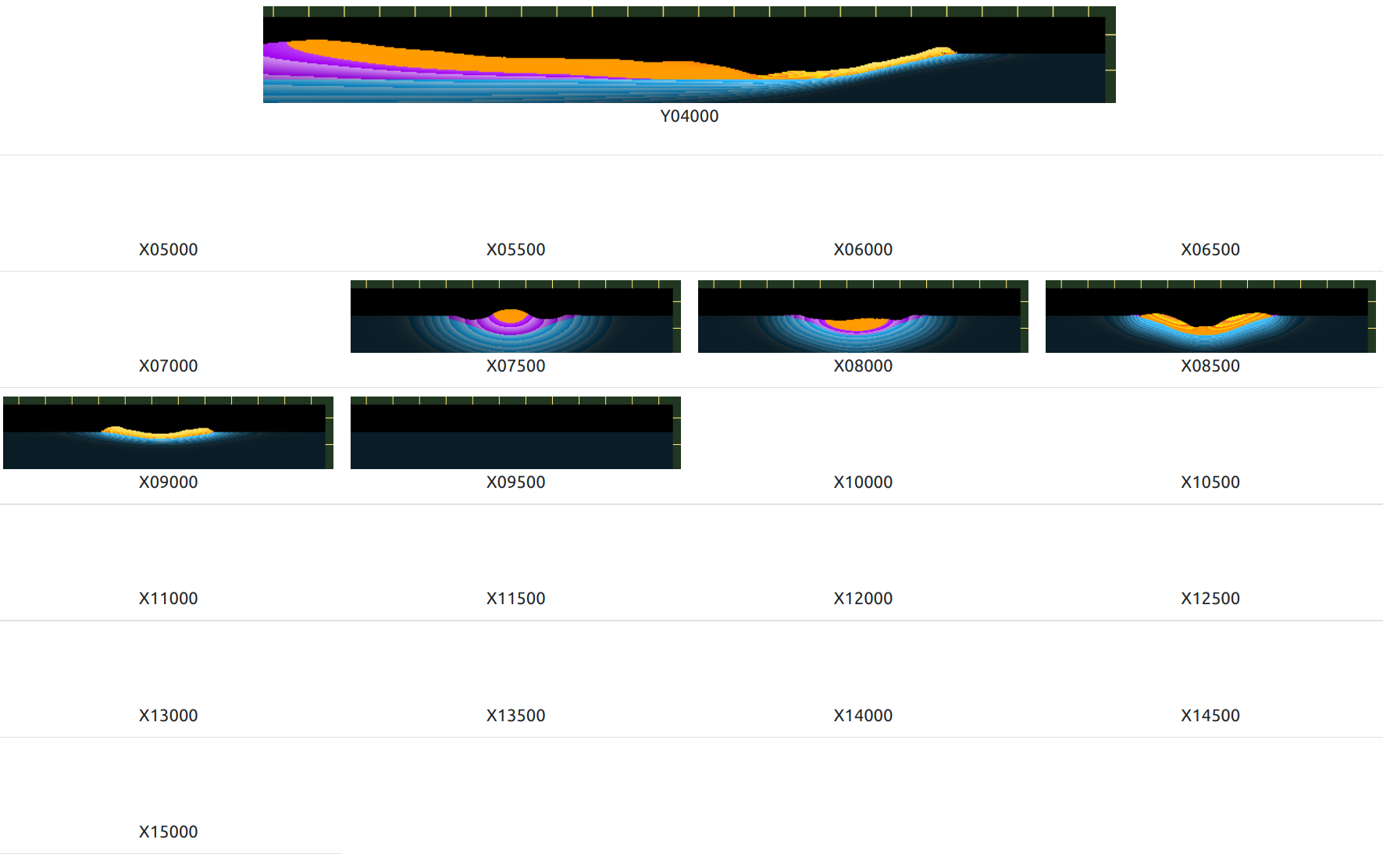
Fig. 26 Example of the output crosssections and the corresponding folder names in the cross-sections directory at the t=66000 time step. The file names of all images are pic66000.png. Orange is fluid, blue is solid, purple is solidified fluid. The visible lines are temperature isocontours. The distance between yellow tics is 100 μm.

The cross-section in the \(x\) – \(z\) plane is in the Y04000 directory, which corresponds to the \(y=4000\) μm coordinate. The cross-section in the \(y\) – \(z\) plane is in the X????? directory, where the name of the directory contains the \(x\) coordiname in μm. The spacing between cross-sections in the output can be adjusted with the Visual.distanceBetweenXsecs parameter in the input JSON file. At the \(t=66000\) time step only the images in the directories X05500 – X09500 are not empty. This is because the images outside the meltpool grid are not rendered. The cross-sections outside the meltpool grid can be rendered from the output geometry file with the use of the drawCrossSection script.

Track analysis

In the simulation folder, run the script generating file geometry data in text format:

> /opt/KiSSAM/scripts/trackAnalyzer.x output/geometry.vdb > track.dat

The output is the text file track.dat.

#units: millimeters
#Xcoord DepthMax HeightMax DepthAtCenter HeightAtCenter WidthMax WidthAtSubstrate
4.896 -0.000999742 0.00200026 -0.000999742 -0.000220794 0.057 -inf
4.899 -0.00699974 0.00220799 -0.00699974 0.000163873 0.081 0.063
4.902 -0.00699974 0.00265304 -0.00699974 0.00198937 0.099 0.087
4.905 -0.00699974 0.00365511 -0.00699974 -0.000998729 0.114 0.108
4.908 -0.00999974 0.00515794 -0.00999974 0.00374949 0.132 0.123
4.911 -0.00999974 0.00705202 -0.00999974 0.00500026 0.138 0.138
...

Here we plot these data

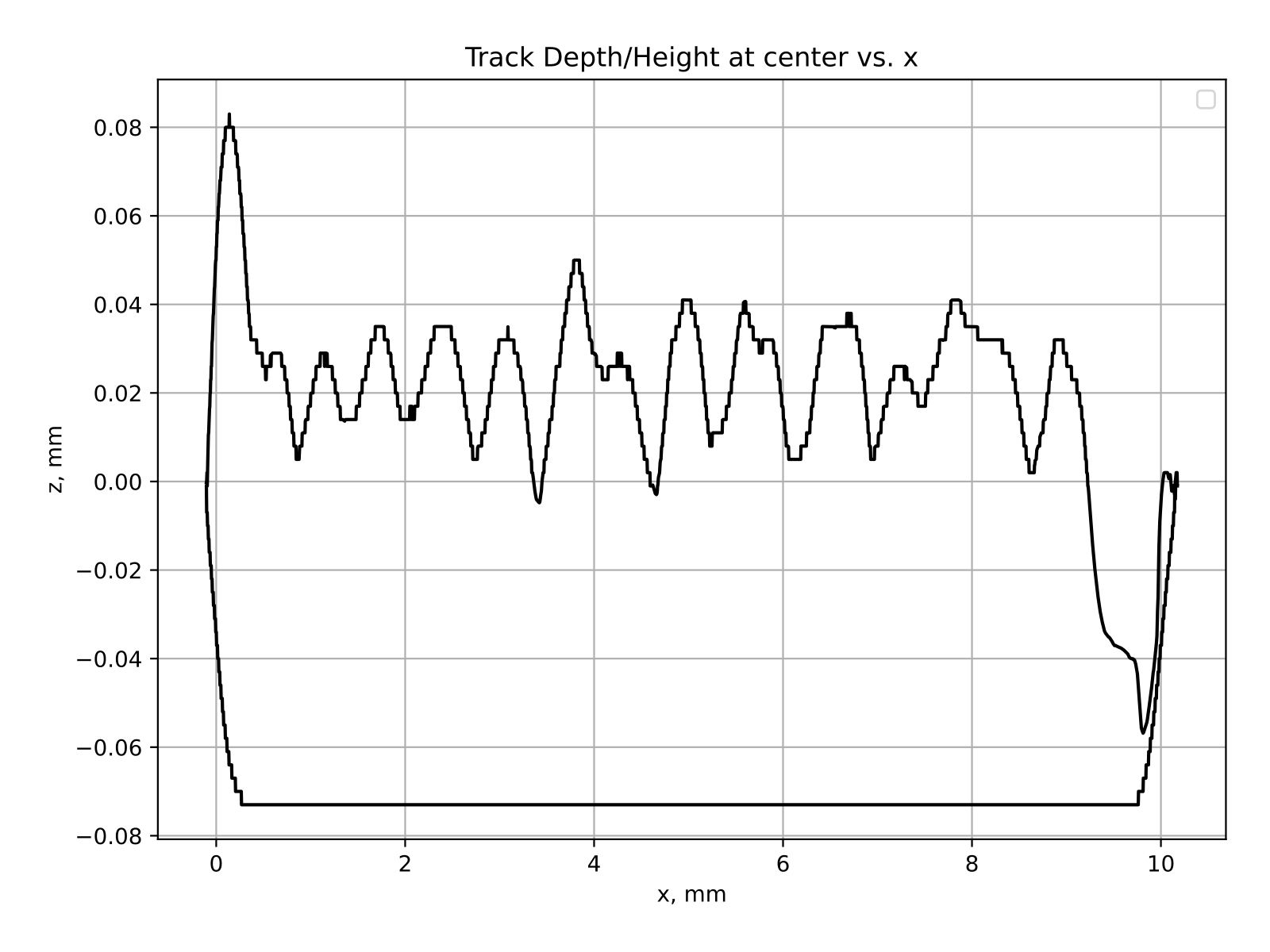
Fig. 27 Track parameters plotted against the scan path direction

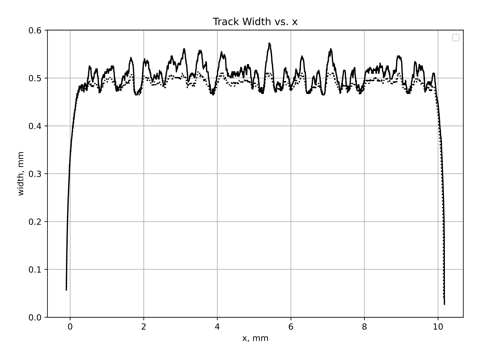
Fig. 28 Track parameters plotted against the scan path direction

Various track statistics, such as mean width (0.5 mm), height (0.024 mm), and depth (0.07 mm) in the stable region can be found by analyzing this file.