Laser Track on Powder Layer

Goal

In this example, simulation of a single track on a powder layer is performed. We take a plate of IN625. The Gaussian laser pulse with normal incidence melts the metal. The laser power is 200W.

Here we vary the laser beam speed to get three modes of melting, including keyhole and shallow melting.

You will need the JSON file provided with the usercase and the pre-made powder geometry file.

Run

Create simulation folder

> mkdir simulation_folder
> cd simulation_folder

Copy the JSON file provided with the usercase into the folder

> mv <path>/Laser_track_powder.json .
> mv <path>/spheresH80-cloned.vdb .

Run the code from terminal with the provided JSON file.

> INPUT_JSON_FILE=Laser_track_powder.json /opt/KiSSAM/start_calc.sh

Make sure that simulation is started by making sure there are no fatal errors in the .log file that has appeared. It might be necessary to insert the correct license filepath.

Input Configuration

While the simulation is running, let us look at the configuration file and see how it may be adjusted.

The simulation parameters can be adjusted by editing the JSON file.

{
  "licenseFile": "/licences/kissam-end-2023-dec.lic",
  "outputDir": "./Speed06/",
  "config": {
    "MaxTimesteps": 320000,
    "DumpDataRate": 32000,
    "IterationSubstepsRate": 500,
    "AutoTermination": true
  },
  "sizes": {
    "FullXapprox": 0.008,
    "FullYapprox": 0.008,
    "FullZapprox": 0.005,
    "substrate"  : 0.00456
  },
  "Powder": {
    "initSpheresVDBfile": "spheresH80-cloned.vdb",
    "wettingAngle": 150
  },
  "Substrate": {
    "preheating"  : 300.0,
    "wettingAngle": 10
  },
  "Material": "In625",
  "ScanStrategy": {
    "Type": "SingleTrack",
    "SingleTrack": {
      "length"   : 5e-3,
      "startPosX": 1.0e-3,
      "startPosY": 2.5e-3
    },
    "Beam": {
      "type"     : "Laser",
      "Shape"    : "Gauss",
      "Power"    : 200.0,
      "Width"    : 100e-6,
      "Speed"    : 0.6
    }
  },
  "Visual": {
    "distanceBetweenXsecs": 0.5e-3,
    "3DrenderedDomainSize": [2e-3, 1.5e-3, 0.5e-3]
  }
}

The scanning track is adjusted in lines 28-30, where its length and coordinates of the starting position are specified in meters. The laser power (W), width (m) and speed (m/s) are set in lines 35-37. The material (line 24) is chosen from the named materials in the materials library.

Here we skip the simulation of powder deposition by taking the pre-made spheresH80-cloned.vdb file.

The parameters that are not specified here are taken from the /opt/KiSSAM/default.json file.

Let us vary the simulation parameters. Change the laser beam speed and the output folder name:

...
"outputDir": "./Speed03/",
...
"Speed"    : 0.3
...

Save the file and run again:

> INPUT_JSON_FILE=Laser_track_powder.json /opt/KiSSAM/start_calc.sh

If the computer has several GPUs, and another GPU is not busy at the moments, the second simulatio is started asynchronously while the first is running.

Let us run one more simulation in the same way, with higher laser beam speed:

...
"outputDir": "./Speed12/",
...
"Speed"    : 1.2
...

Simulation Results

The simulation runs for ~6 hours. In our simulation folder, there will be three directories with the output of the three simulations.

3D view

The track geometry is stored in the openVDB format output/geometry.vdb. It is updated during the simulation process and stores the latest state. View it with Blender or VDB view.

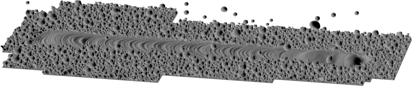
Fig. 29 Speed 0.3 m/s

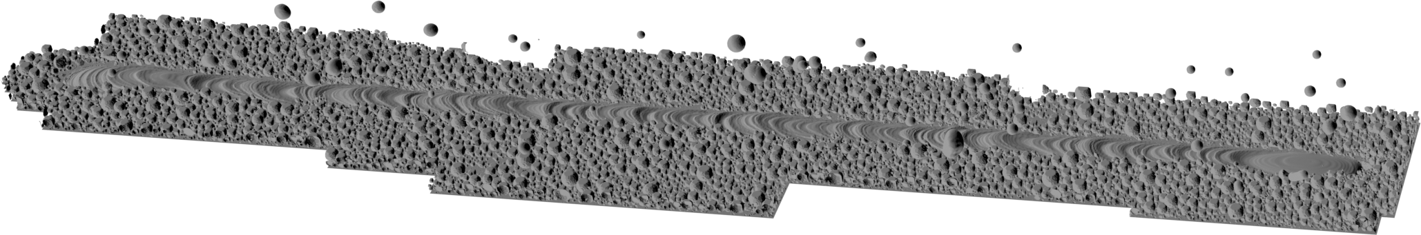
Fig. 30 Speed 0.6 m/s

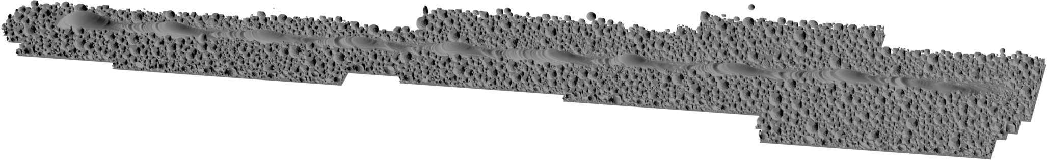
Fig. 31 Speed 1.2 m/s

Melt pool Statistics

The evolution of the size of the melt pool can be found in the text file meltpoolStats.dat. Here are the plots from the columns WidthX, WidthXatSubstrate, WidthXatBeam of that file in each of the simulation directories:

Fig. 32 Melt pool length in the scanning direction

Images output

The meltpool states are rendered as images and stored in output/rendered3D. The images of cross-sections are found in output/cross-sections. Let us compare the y cross sections in the three simulations. Let us take a time instant where the meltpool shape has reached a stable shape during the scanning \(t=3\) ms. The time step is \(3\cdot 10^{-8}\), thus we look at the output of the 100 000th iteration:

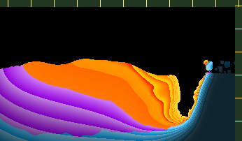
Fig. 33 Speed 0.3 m/s, file /Speed03/cross-sections/Y02500/sec-it000100000.png

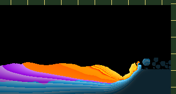
Fig. 34 Speed 0.6 m/s, file /Speed06/cross-sections/Y02500/sec-it000100000.png

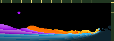
Fig. 35 Speed 1.2 m/s, file /Speed12/cross-sections/Y02500/sec-it000100000.png

Track analysis

In the simulation_folder, run the script that generates a file with track parameters:

> /opt/KiSSAM/scripts/trackAnalyzer.x Speed03/geometry.vdb > speed03_track_parameters.txt
> /opt/KiSSAM/scripts/trackAnalyzer.x Speed06/geometry.vdb > speed06_track_parameters.txt
> /opt/KiSSAM/scripts/trackAnalyzer.x Speed12/geometry.vdb > speed12_track_parameters.txt

The output is the text file track_parameters.txt.

#units: millimeters
#Xcoord DepthMax HeightMax DepthAtCenter HeightAtCenter WidthMax WidthAtSubstrate
0.939 -0.000999742 0.00200026 inf -inf 0.021 -inf
0.942 -0.000999742 0.00222667 -0.000999742 -0.00020045 0.042 -inf
0.945 -0.000999742 0.00200026 -0.000999742 -0.00010976 0.057 -inf
0.948 -0.000999742 0.00201591 -0.000999742 -0.000409314 0.075 -inf
...

Here are plots DepthAtCenter(Xcoord), HeightAtCenter(Xcoord):

Fig. 36 Minimal and maximum \(z\) coordinate of the meltpool at the track center vs \(x\)

As expected, lower laser beam speed leads to a deeper melt. Few peaks in the image are caused by the flying liquid droplets.

Energy Absorbtion Diagnostics

The energy absorbtion data is written to the absorbedEnergy.dat file. To find the ratio of the absorbed energy, take the sum of the BeamPowerFluid and BeamPowerSolid columns, divide by the total laser power (the ScanStrategy.Beam.Power parameter in the JSON file), and divide by the time the power was being recorded (the config.IterationSubstepsRate field in the JSON file).

\[\frac{\texttt{BeamPowerFluid}+\texttt{BeamPowerSolid}} {TP}\]

Here, \(T=\texttt{config.IterationSubstepsRate}=500\) and \(P=\texttt{ScanStrategy.Beam.Power}=200\) W.

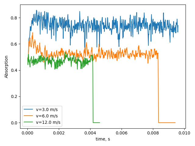
Fig. 37 The absorbtion vs time for the three cases.