Laser Track on Flat Substrate

Goal

In this example, simulation of a single track on a bare plate in the “keyhole” regime is considered. We take a plate of IN625. The Gaussian laser pulse with normal incidence melts the metal. The laser scan speed is 0.4 m/s, power is 150W.

You will need the JSON file provided with the usercase.

Run

Create simulation folder

> mkdir simulation_folder
> cd simulation_folder

Copy the JSON file provided with the usercase into the folder

> cp <path>/Laser_track_plate.json .

Run the code from terminal with the provided JSON file.

> INPUT_JSON_FILE=Laser_track_plate.json /opt/KiSSAM/start_calc.sh

Make sure that simulation is started by making sure there are no fatal errors in the .log file that has appeared. It might be necessary to insert the correct license filepath in the appropriate field in the JSON file.

Input Configuration

While the simulation is running, let us look at the configuration file and see how it may be adjusted. If you want to adjust the parameters, make sure that the simulation is stopped or finished. Before restrating the simulation with a new file, if you want to keep the previous results, make sure to specify another directory for the output (the outputDir parameter).

The user defined simulation parameters are in the input JSON file.

{
  "licenseFile": "/licences/kissam-end-2023-6-30.lic",
  "config": {
    "MaxTimesteps"         : 300000,
    "DumpDataRate"         : 30000,
    "IterationSubstepsRate": 1000
  },
  "NumericalParams": {
    "dr"       : 3e-6,    
    "dt"       : 30e-9
  },
  "Substrate": {
    "preheating"  : 300.0,
    "wettingAngle": 10
  },
  "Material": "In625",
  "ScanStrategy": {
    "Type": "SingleTrack",
    "SingleTrack": {
      "length"   : 3e-3,
      "startPosX": 1e-3,
      "startPosY": 2e-3
    },
    "Beam": {
      "type"     : "Laser",
      "Shape"    : "Gauss",
      "Power"    : 150.0,
      "Width"    : 100e-6,
      "Speed"    : 0.4
    }
  },
  "Visual": {
    "distanceBetweenXsecs": 500e-6,
    "3DrenderedDomainSize": [2e-3, 1.5e-3, 0.5e-3]
  }
}

Scanning track is adjusted in lines 20-22, where its length and coordinates of the starting position are specified in meters. Laser power (W), width (m) and speed (m/s) are set in lines 27-29. Material (line 16) is chosen from the named materials in the materials library.

The parameters that are not specified here are taken from the /opt/KiSSAM/default.json file. The full list of parameters that were taken in the simulation can be found in the full_params.json file in the output directory.

Simulation Results

The simulation runs for ~2.5 hours. The default name for the simulation output directory is output.

3D view

The track geometry is stored in the openVDB format output/geometry.vdb. It is updated during the simulation process and stores the latest state. View it with Blender or VDB view.

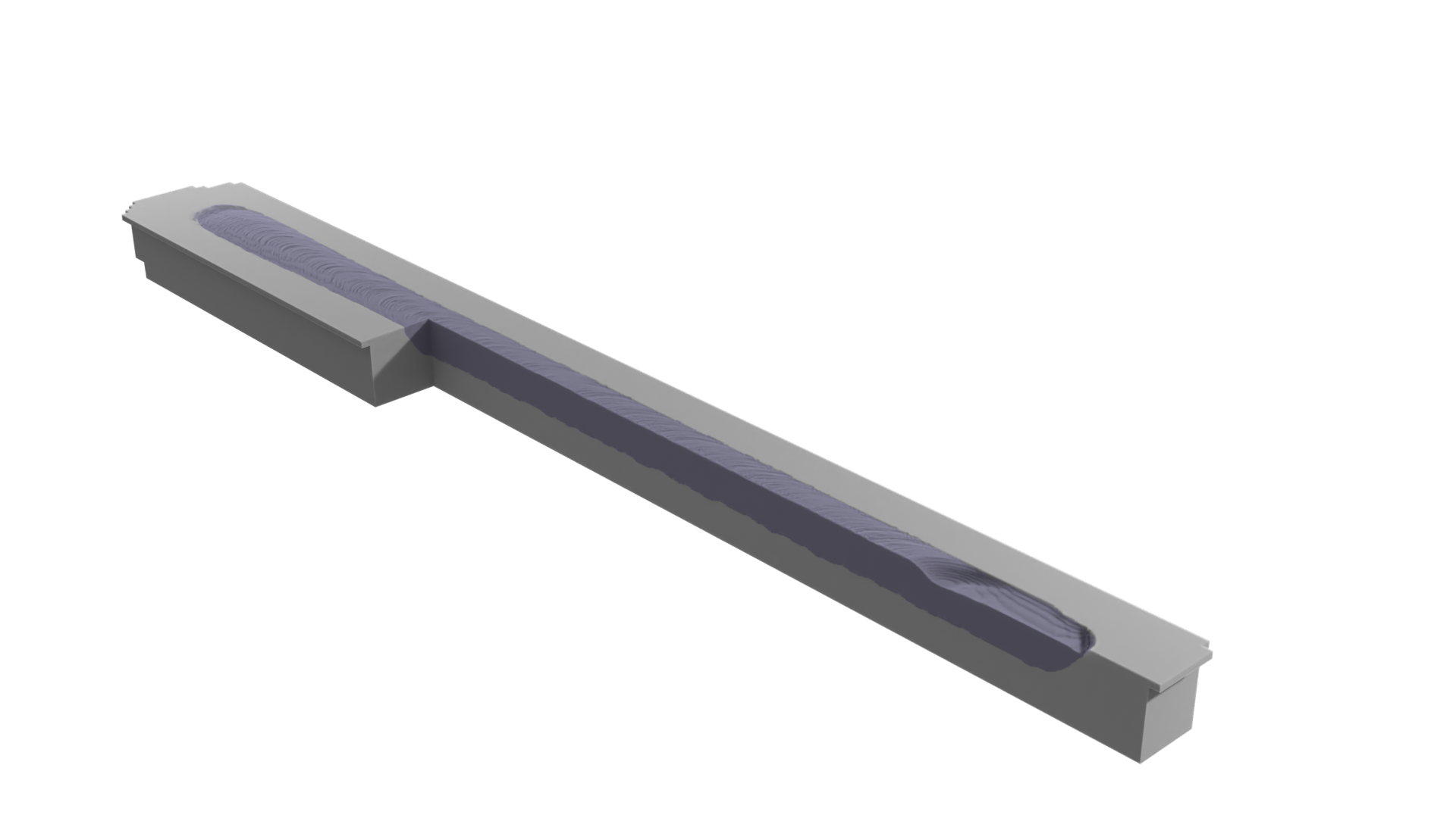
Fig. 22 openVDB file loaded and rendered in Blender

Images and animation output

The melt pool states are rendered as images and stored in output/rendered3D. The images of cross-sections are found in output/cross-sections.

In the simulation_folder, run the script generating one image from several cross-sections.

> /opt/KiSSAM/scripts/combine_images.sh output --overlay --dr 3

The generated images are placed in the combinedIMG folder in the simulation_folder/output. The images are combined into a movie and written to combinedIMG/video.wmv.

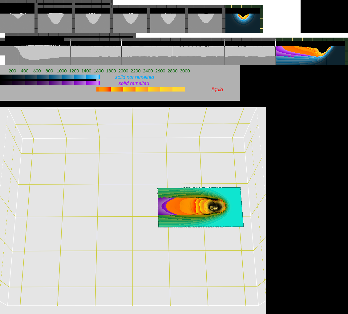
Fig. 23 Example of the combined image combinedIMG/pic-250000.png

Melt pool Statistics

The evolution of the size of the melt pool can be found in the text file meltpoolStats.dat. Here are plots from the columns of the file:

Fig. 24 Melt pool height and depth, measured from substrate. The total vertical size of the melt pool is height+depth.

Fig. 25 Melt pool length in the scanning direction.

Fig. 26 Melt pool width.

The characteristic geometry is estimated in the area of stable scanning, where the effects of the beginning and the end of the track are not seen. Here are statistics from \(t=0.003\) to \(t=0.006\) s:

Depth	\(9.8\cdot 10^{-2}\) mm
Height	\(4.0\cdot 10^{-3}\) mm
Length	\(4.8\cdot 10^{-1}\) mm
Width	\(0.15\) mm

Track analysis

In the simulation_folder, run the script that generates a file with track parameters:

> /opt/KiSSAM/scripts/trackAnalyzer.x output/geometry.vdb > track_parameters.txt

The output is the text file track_parameters.txt.

#units: millimeters
#Xcoord DepthMax HeightMax DepthAtCenter HeightAtCenter WidthMax WidthAtSubstrate
0.939 -0.000999742 0.00200026 inf -inf 0.021 -inf
0.942 -0.000999742 0.00222667 -0.000999742 -0.00020045 0.042 -inf
0.945 -0.000999742 0.00200026 -0.000999742 -0.00010976 0.057 -inf
0.948 -0.000999742 0.00201591 -0.000999742 -0.000409314 0.075 -inf
...

Here are plots DepthAtCenter(Xcoord), HeightAtCenter(Xcoord), WidthMax(Xcoord):

Fig. 27 Minimal and maximum \(z\) coordinate of the meltpool at the track center vs \(x\).

Fig. 28 Difference between the minimal and the maximal \(y\) coordinate of the meltpool vs \(x\).

Here are the mean values in the \(x=1.3\) mm to \(x=2.2\) mm range from the track start:

Depth	\(0.10\) mm
Height	\(0.004\) mm
Width	\(0.15\) mm

Cross Section Image

Let us compare with the experimental images. In [Lane, B., Heigel, J., Ricker, R. et al. Measurements of Melt Pool Geometry and Cooling Rates of Individual Laser Traces on IN625 Bare Plates. Integr Mater Manuf Innov 9, 16–30 (2020)] there is a published image of the track cross section:

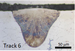
Fig. 29 Cross section photo from experimental data

Let us run this script to extract cross-section at \(x=1.5\) mm from the track start startPosX (\(1\) mm). To get a cross-section at the right place, let us look at the position of the track in the simulation domain. If these parameters were not in the user defined JSON, they were taken from the default settings. The exact parameters that were used in the simulation can be found in the full_params.json file in the output directory. Here we have:

...
"sizes" => {
    "FullXapprox" => 0.005 &&&
    "FullYapprox" => 0.005 &&&
    "FullZapprox" => 0.004 &&&
    "substrate" => 0.0035 &&&
...
   "ScanStrategy" => {
    "Type" => "SingleTrack" &&&
    "SingleTrack" => {
        "length" => 0.003 &&&
        "startPosX" => 0.001 &&&
        "startPosY" => 0.002
...

The \(z\)-axis range should be around the substrate (3.5 mm). Let us take the range from (substrate-Depth) to (substrate + Height) with some margin. Depth (0.1 mm) and height (0.004 mm) are taken from the track analysis above.

The \(y\)-axis range should be around the track \(y\)-axis position (2 mm). The width can be estimated from the track analysis above, or from the beam width.

> /opt/KiSSAM/scripts/drawCrossSection.x output/geometry.vdb trackXcrossSection.png --box 2.5,1.90,3.38 2.5,2.09,3.5 --background E8F0F200 --substrate 295569FF --remelted CD86F2FF

One pixel of the image is one mesh step: NumericalParams.dr (3 μm) in the input file.

Fig. 30 Cross section in the simulation.