SCRIPTS

Introduction

The are some typical scenarios of working with input and output data of KiSSAM. The software package includes a variety of scripts for pre- and postprocessing.

The scripts are used through the Linux command line. To use a script, the following patters should be written in the bash terminal

<script name> <option(s)> <arguments(s)> [<optional argument(s)>]

The <script name> includes the path to the KiSSAM instalation folder. In the instructions below, we use angle brackets to indicate arguments that should be filled in, and square brackets to indicate optional arguments.

Simulation Preparation Scripts

Powder Sphere Rasterization

rasterizeSpheres.x rasterizes spheres from text list into the VDB format. VDB file contains volumetric data: the filling fraction of material on a fine mesh. Usage:

/opt/KiSSAM/scripts/rasterizeSpheres.x  <VoxelSize> <file>

<file> (for example, spheres.dat) should be a text file with the four columns: \(x\), \(y\), \(z\) coordinates of the sphere position and radius (in micrometers). <VoxelSize> is the mesh step size in micrometers.

27.4911 27.4917 27.4911 27.5
44.7133 79.1247 63.0167 37.5
87.07 32.4956 32.4953 32.5
166.9 34.6008 27.4979 27.5
128.672 75.4377 27.498 27.5
...

After that the file init_spheres.vdb will be created. To use it in the simulation, specify its name and file path in the JSON field Powder.initSpheresVDBfile. Make sure that the mesh step size in the KiSSAM simulation configuration (default.json, or the input JSON) in NumericalParams.dr is equal to <VoxelSize> specified here. Note that NumericalParams.dr is specified in meters, while <VoxelSize> is specified in micrometers.

Post Processing Scripts

Visualization helpers

Combine images

During the simulation, images are written into the rendered3D directory, as well as several subdirectories in the cross-sections/ directory. To combine the images that correspond to one time instant in one image, use the combine_images.sh script.

/opt/KiSSAM/scripts/combine_images.sh <simulation_directory> [--overlay] [--dr <dxstep>]

The arguments in the square brackets are optional.

-dr <dxstep>

Specify the pixel size in micrometers. Should be equal to the NumericalParams.dr used in the simulation. If the option is added, the lines at Y-section image at correct places of X-sections are drawn over the image.

--overlay

If this option is used, the combined image has not only all the images on the current time, but also the images on the previous times. The current image always contains only the melt pool region. To see the previously solidified images as well, turn on --overlay.

Example. In the directory, where the simulation was started, execute the command:

/opt/KiSSAM/scripts/combine_images.sh output --overlay

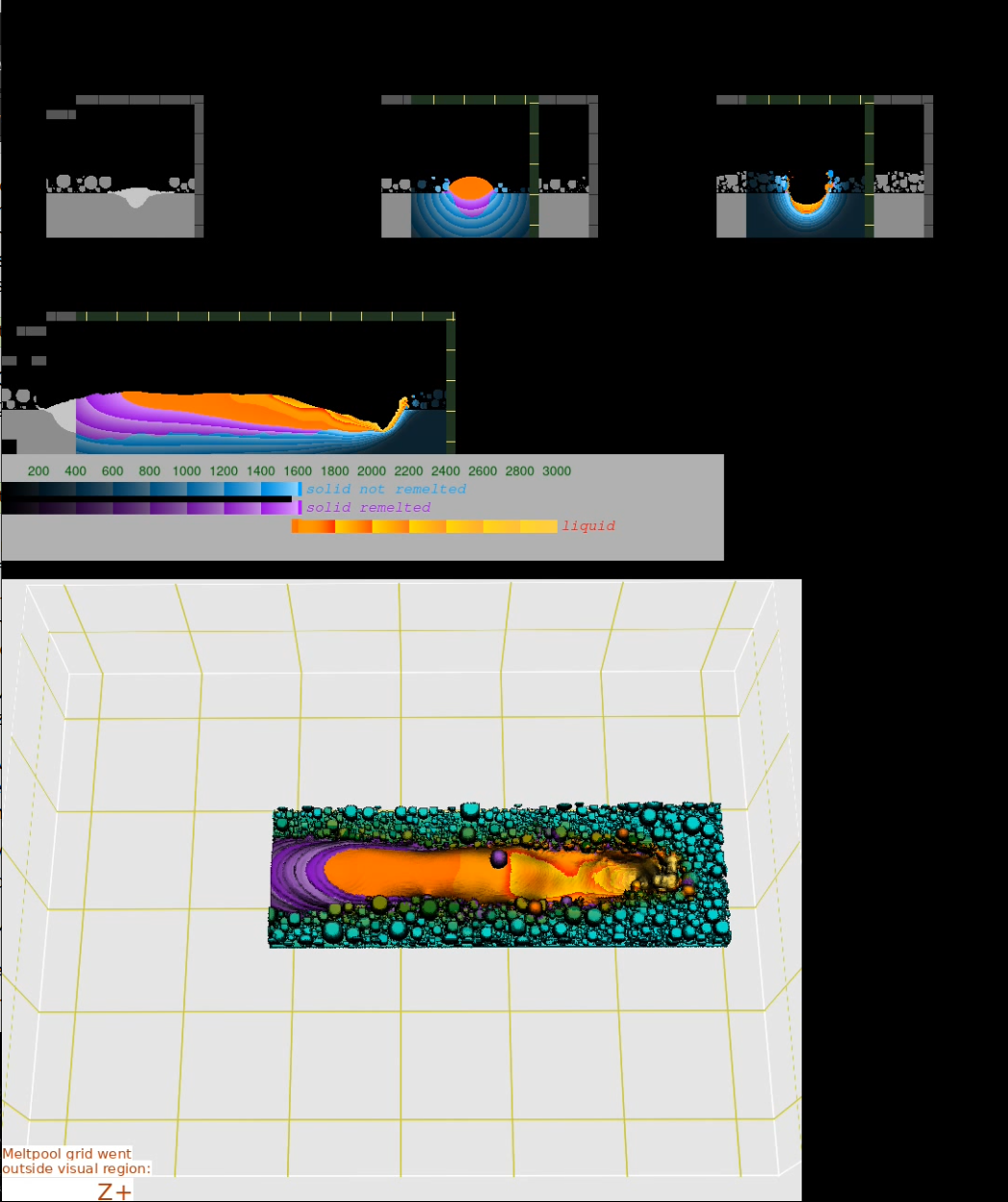
Fig. 6 Result of the script with the overlay option.

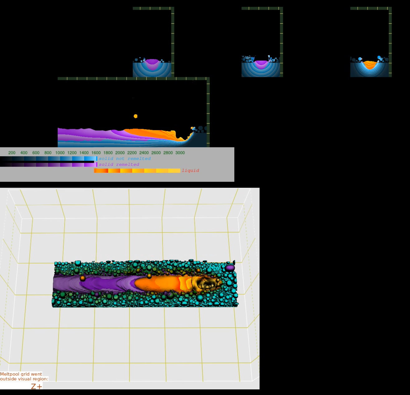
Fig. 7 Result of the script without the overlay option.

The result is written in the output/combinedIMG folder. At the same time, the animation of the images is generated and can be found in the output/combinedIMG/video.wmv file. Note that picture files in the cross-sections/ and rendered3D/ directories must have correct file names with cycle iteration ratio of 1000.

Pad images

Since the meltpool grid adapts to the size of the meltpool, the images in different time steps have different sizes. This is inconvenient for many purposes, such as animations and slideshows. Moreover, the cross sections in the planes with no melted material are often represented with empty images. The pad_images.sh script creates images with equal width and length and easily to batch them in video later. This script is used by the combine_images.sh script.

Generate Cross Section Images

The script drawCrossSection.x generates cross-sections pictures from the geometry.vdb file. Usage:

./drawCrossSection.x geometry.vdb [ section-pic.pam | section-pic.png ] --sec x|y|z coordinate | --box Xmin,Ymin,Zmin Xmax,Ymax,Zmax
                        [ --autoclip ]
                        [ --grains ]
                        [ --hl_bound_grains ]
                        [ --background COLOR ]
                        [ --substrate COLOR ]
                        [ --powder COLOR ]
                        [ --remelted COLOR ]
                        [ --smooth ]
                        [ --comp_limit lim1,lim2 ]
                        [ --comp_color COLOR ]

Output image file should be specified either with .pam or .png extenstion.

The section can be set either with the --sec option or with the --box option. All the values must be specified in millimeters units.

If the --sec option is used, one of x, y or z symbols should be chosen and the coordinate should be given. The cross section is taken on that coordinate

If the --box option is used, one, and only one of the following conditions must be fullfied: xmin == xmax, or ymin == ymax or zmin == zmax. If xmin == xmax, the output image <output-picture.ppm> is a section of the geometry where ymin\(<y<\) ymax, zmin\(<z<\) zmax. Cross sections in the other two perpendicular planes are made if zmin == zmax or ymin == ymax.

--autoclip

Crop the area where there is no remelted geometry

--grains

Color the grains if the grain growth model for simulation of microstructure was turned on in the simulation

--hl_bound_grains

Highlight the grain boundaries with solid lines

--background

After this option, specify the color of the image background in the HEX format. Default is 000000FF

--substrate

Color of the substrate in the initial geometry. Default is 7F99B2FF

--powder

Color of the powder. Default is 7F99B2FF

--remelted

Color of the melted material. Default is 33E5FFFF

--smooth

Enable anti-aliasing for the surface

--comp_limit

For multicomponent evaporation simulation, set the limits of the first component for visualization

--comp_color

For multicomponent evaporation simulation, set the color of the component. The color is added to the color of the substrate or powder.

Colors are in the RGBA format and can be transparent.

Here is an example how the --box option is used:

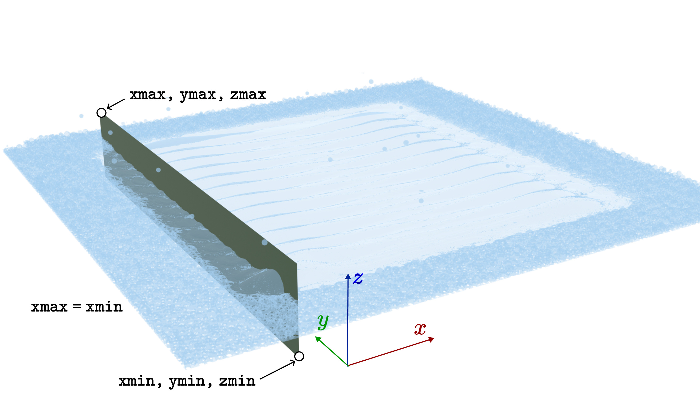
Fig. 8 Illustration of the box parameters.

Fig. 9 Cross section result from the previous figure

Here is an example. Let us plot cross section for the simulation which was run with the following data in the input JSON file:

 "sizes": {
  "FullXapprox": 0.008,
  "FullYapprox": 0.008,
  "FullZapprox": 0.005,
  "substrate"  : 0.00456
},
"ScanStrategy": {
  "Type": "SingleTrack",
  "SingleTrack": {
    "length"   : 5e-3,
    "startPosX": 1.0e-3,
    "startPosY": 2.5e-3
  },

To plot the cross section along the track, we have to specify the \(y=2.5\) mm plane. Thus, ymin = 2.5 = ymax. The cross section box has be around the substrate: zmin < 4.56 mm < zmax. The box has to include the length of the track:xmin < 1 mm < 1+5 mm < xmax. We run the command with

/opt/KiSSAM/scripts/drawCrossSection.x drop/geometry.vdb longCrossSection.png --box 0,2.5,4.4 7,2.5,5

And get the result

Here is an example with specified colors:

/opt/KiSSAM/scripts/drawCrossSection.x drop/geometry.vdb longCrossSection.png --box 0,2.5,4.4 7,2.5,5 --background  00000000 --substrate 7F6D94FF --powder 295569FF --remelted CD86F2FF

Geometry Post-Processing

Activate Grids

Some of the output VDB files contain grids with all the data, but the cells are not activated, and can not be visualized. In the output geometry VDB file, only the cells that were in the fluid simulation domain are activated, and some of the stationery geometry will not be visualizaed. Use the activateGrids.x script to activate the grids.

/opt/KiSSAM/scripts/activateGrids.x <geometry-input.vdb> <geometry-output.vdb> [--crop <Xmin,Ymin,Zmin Xmax,Ymax,Zmax>]

Rendering of the file with activated geometry can take longer time.

--crop

The option --crop can be used to decrease file size. With it, only the box specified by two corners Xmin < \(x\) < Xmax, Ymin < \(y\) < Ymax, Zmin < \(z\) < Zmax (in mm) is written to the output file.

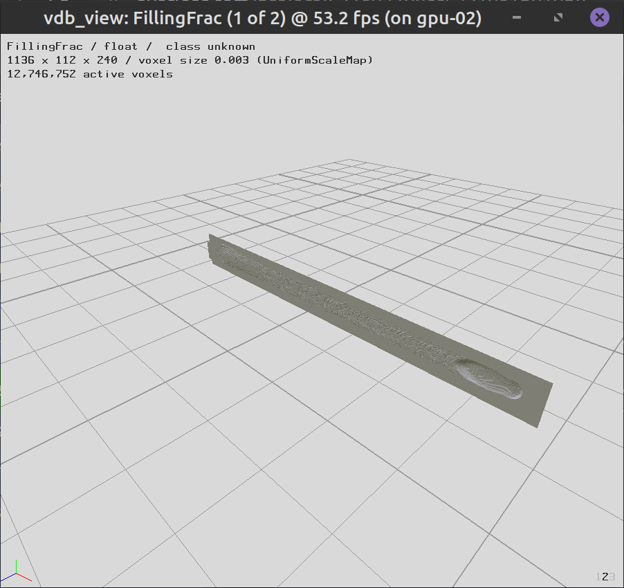
Fig. 10 Before

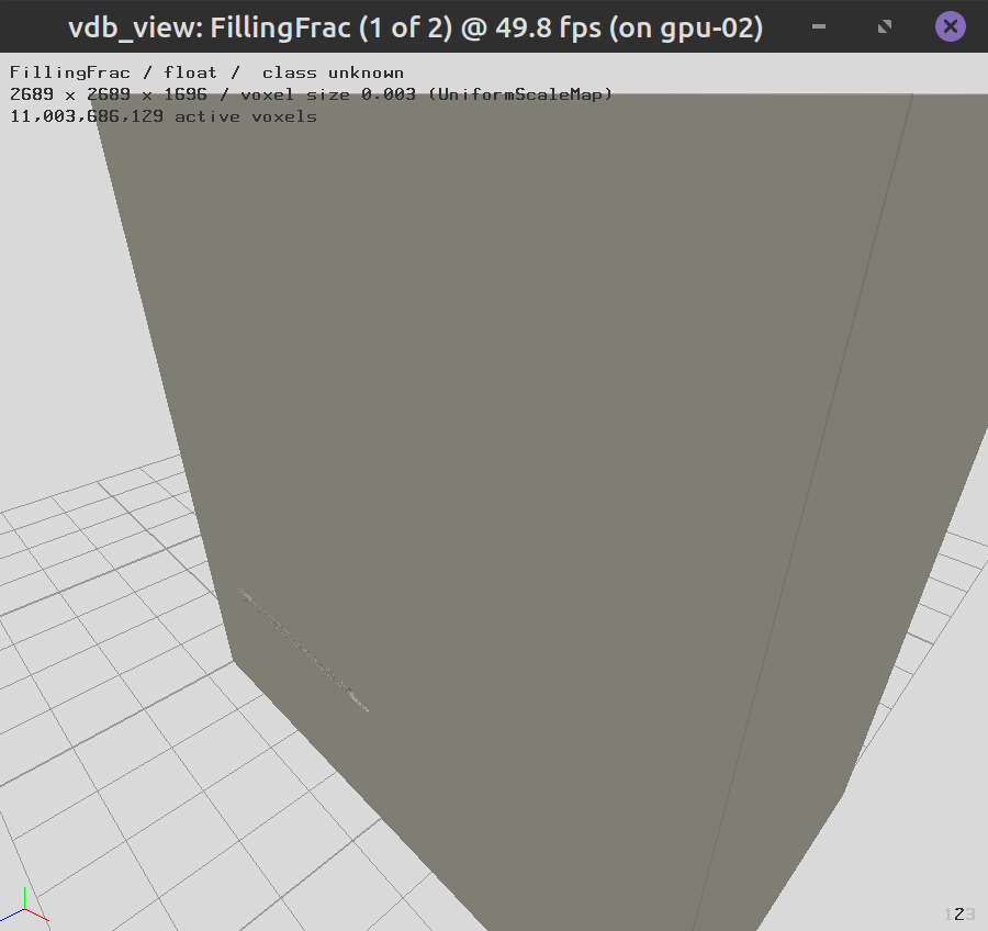
Fig. 11 After

Remove Isolated Geometry

The script removeIsolated.x removes isolated spatters from geometry.vdb file which are not connected with resulted solidified surface. Usage:

/opt/KiSSAM/scripts/removeIsolated.x geometry.vdb sim_geometry.vdb

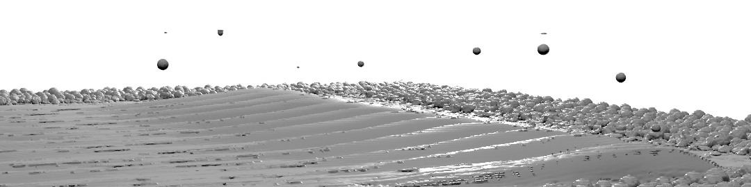
Fig. 12 Before (geometry.vdb)

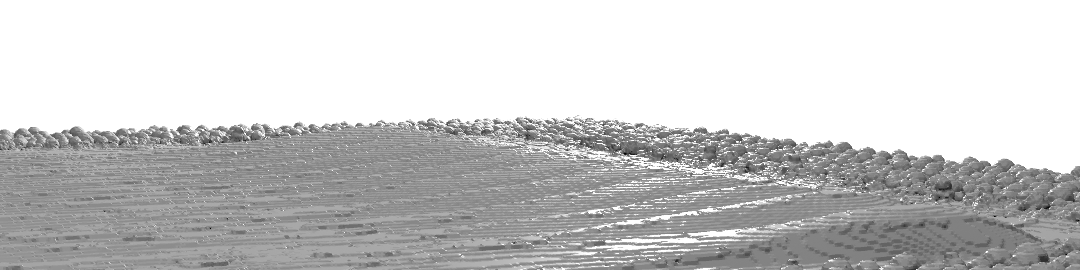
Fig. 13 After (sim_geometry.vdb)

Remove Powder

To study a finished sample after the multilayer simulation is complete, run the removePowder.x script.

/opt/KiSSAM/scripts/removePowder.x

Merge Layers

In a multi-layer simulation, the latest geometry.vdb file treats only the last layer as melted and solidified material, and all previous layers as initial substrate. To find all melted and solidified material across several layers in one VDB file, use the mergeLayers script.

Usage:

./mergeLayers.x <vdb_file1.vdb> <vdb_file2.vdb> <vdb_file3.vdb> ... [--remelted input_files*.vbd] --out <output_file.vdb> [--debug]

--remelted

If the --remelted option is specified, in this case the remelted regions will be picked up only from the selected files.

--secern

If the --secern option is specified, the remelted part of different vdb files will be marked with a different value in the ParticleIds grid in the resulting VDB file.

Convert into Triangulated 3D Surface

The script vdb2stl.x creates an STL-file of the surface geometry (based on the FillingFrac field of the VDB file). Usage:

/opt/KiSSAM/scripts/vdb2stl.x <vdb_file> <stl_file>  [--only-active]

The output file size is often very large.

--only-active

To suppress non-active regions run with the --only-active option.

To reduce the file size by simplifying geometry, use the decimate_stl.py script.

Simplify Surface

The script decimate_stl.py decimates an STL file (reduces the total number of polygons). This is used to prepare a cost-efficient input for the powder generation software.

python3 /opt/KiSSAM/scripts/decimate_stl.py surface.stl

Cleanup Surface

Process STL file to remove all internal triangles.

/opt/KiSSAM/scripts/stlHull.x

Geometry Diagnostics

Track geometry analysis

Use the script trackAnalyzer.x to extract some information about single track from output geometry.vdb file. Simulation parameters that are needed to extract length scale for the use in this script, are in the metadata of the geometry.vdb file.

The script prints into stdout the following x-axis dependent parameters of the track: maximal track depth and height, depth and height at the center, maximal width and width at substrate level.

Usage:

/opt/KiSSAM/scripts/trackAnalyzer.x <VDB file> > <output file>

The script works correctly if scanning strategy ScanStrategy.Type was set to SingleTrack. This strategy implies scanning along \(x\)-axis.

On the cross-sections where \(x=\) Xcoord, the following quantities are found

Key	Description
Xcoord	\(x\) axis coordinate (mm)
DepthMax	the (signed) distance from the lowest point of the solidified metal to the surface (mm)
HeightMax	the (signed) distance from the highest point of the solidified metal to the surface (mm)
DepthAtCenter	the (signed) distance from the lowest point of the solidified metal in the center of the track (fixed \(y\)) to the surface (mm)
HeightAtCenter	the (signed) distance from the highest point of the solidified metal in the center of the track (fixed \(y\)) to the surface (mm)
WidthMax	maximal width of the melted metal in the center of the track (mm)
WidthAtSubstrate	the width of the melted metal in the center of the track, measured at substrate surface (mm). Inf if there is no melted metal in this position

Analyze Surface

The surfaceAnalyzer.x script outputs a 3D surface as a height function of coordinates \(h(x,y)\) in the text file format.

/opt/KiSSAM/scripts/surfaceAnalyzer.x sim_geometry.vdb > groundsurf.dat

The groundsurf.dat file contains height as a \(h(x,y)\) table, and melted material depth in the same format. Here is an example

#units: millimeters
#Xcoord Ycoord SurfaceHeight MeltpoolDepthPosition
0 0 4.564 4.564
0.007 0 4.564 4.564
0.014 0 4.564 4.564
0.021 0 4.564 4.564
0.028 0 4.564 4.564
0.035 0 4.564 4.564
...

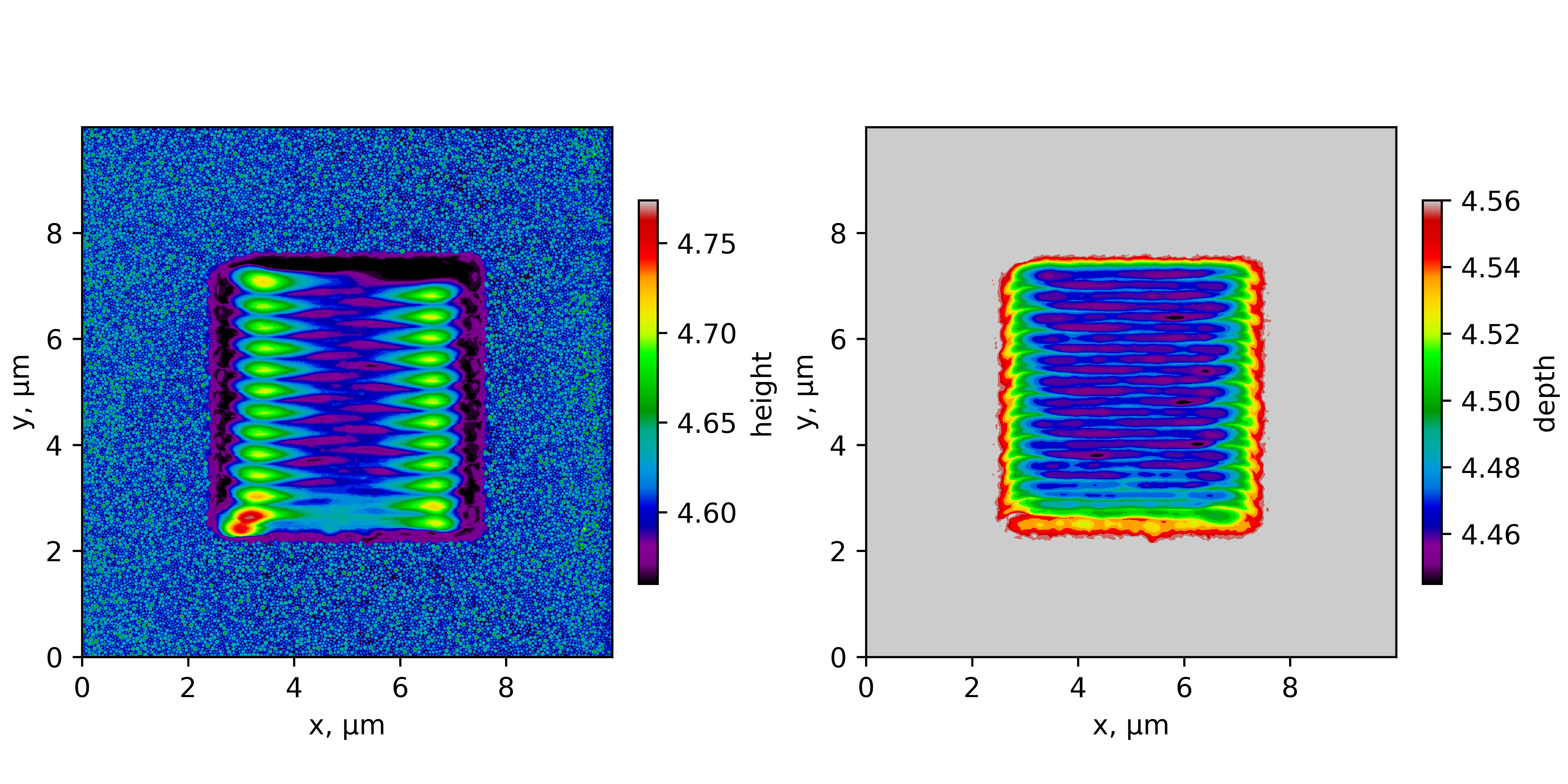
Fig. 14 Surface plot of the script output.

Analyze Porosity

The ./calcPorosity.x calculates volume and porosity map of the bulk material. Usage

/opt/KiSSAM/scripts/calcPorosity.x geometry.vdb [ --voxel_size <vx,vy,vz> ] [ --box <Xmin,Ymin,Zmin Xmax,Ymax,Zmax> ] [ --obviate_above ]

Coordinates units are millimeters. The geometry is subdivided into rectangles with the size voxel_size. The averaged porosity over each rectange is written to the output.

--voxel_size

Voxel sizes are specified in mm. Voxel sizes can be set as -1. In that case, the full grid size along axis is assumed. Default voxel sizes are -1,-1,-1, and one porosity value for the whole region is computed.

--box

Analyze porosity only in specified box (box sizes are specified in mm).

--obviate_above

Do not consider the void region above the powder/remelted material as special region without pores.

Sample usage:

/opt/KiSSAM/scripts/calcPorosity.x drop/geometry.vdb --voxel_size 0.03,-1,-1

After the computation is finished, the output contains several columns, as in

#X-coordinate(mm) TotalVolume(mm^3)   RemeltedVolume(mm^3)    TotalBulkDensity,%

 ...
1.185 1.200390        0.000537        91.42789
1.215 1.200390        0.000539        91.48217
1.245 1.200390        0.000515        91.45513
1.275 1.200390        0.000505        91.48800
1.305 1.200390        0.000531        91.46917
1.335 1.200390        0.000528        91.46649
1.365 1.200390        0.000486        91.41384

The melted material in geometry.vdb is only the material melted in the latest layer. In case the porosity across several layer is required, use the mergeLayers.x script in advance.

Analyze grains microstructure

The script is used to output a table with analysis of the grains.

Usage:

/opt/KiSSAM/scripts/statGrains.x geometry.vdb gtable.dat

Here, geometry.vdb is the result of KiSSAM simulation with grains growth model turned on, and gtable.dat is a text file, where each line corresponds to one grain.

The text file contains the header where the content of the columns is explained. For each grain, there is a row which contains:

• The center of mass;

• Volume;

• Half axes of the equivalent inertia ellipsoid (a, b, c), in the increasing order. ;

• Axes of the inertia ellipsoid (3 vectors), which correspond to the a, b and c half axes;

• Euler angles of the crystallographic grain orientation;

• The remelted flag, which states if the grain has been remelted (None, Partially, or Fully);

• The isBoundary flag, which states if the grain is at boundary of the domain, or at the boundary defined in the sizes.GrainsLimitBox parameter in the JSON file.

The script has the options:

--only-remelted

Only the grains which were remelted at least partially are analyzed

--ignore-boundary

будут выводиться только зерна, у которых флаг IsBoundary = No

If the statistics is needed in the portion of the domain, the geometry.vdb file can be preprocessed with the Activate Grids scripts with the –crop option. This method can be used to output statistics of a 2D slice.