
Web Version
Introduction
A trial version of KiSSAM is available for free. Contact us or fill in the form on the homepage. The trial version is installed as a cloud service. We pay for the costs of the cloud service so you can try out our software, therefore, the simulation time is very limited. Nevertheless, the provided time is enough to model many scanning setups, due to the high performance of our package.
The trial version has web interface, so the simulation can be controlled remotely from any device with a web browser. However, in it, you can adjust only a small portion of the simulation parameters, and run a limited number of post-processing scripts. This page gives an introduction for the work in the web-based graphical user interface of the trial KiSSAM cloud service.
We appreciate all feedback from our users. Please write us with any thoughts and comments on your experience with our software. If you encounter any problems, the issue is easier to resolve if you write us as soon as possible. For communication, answer the emails that contained your login detail, and refer to your calculation IDs.
In the default simulations with laser source, the time step is 30 ns, the smallest mesh step is 3 micrometers (except for “AA5182”,”AlSi10Mg” materials). In the simulation with electron beam source, the time step is 75 ns, the smallest mesh step is 5 micrometers.
We can adjust default settings for the web users through personal requests.
Setting parameters and initializing the calculation
The user selects the calculation type on the page shown below, provides a name, and creates a simulation page (Create Simulation).
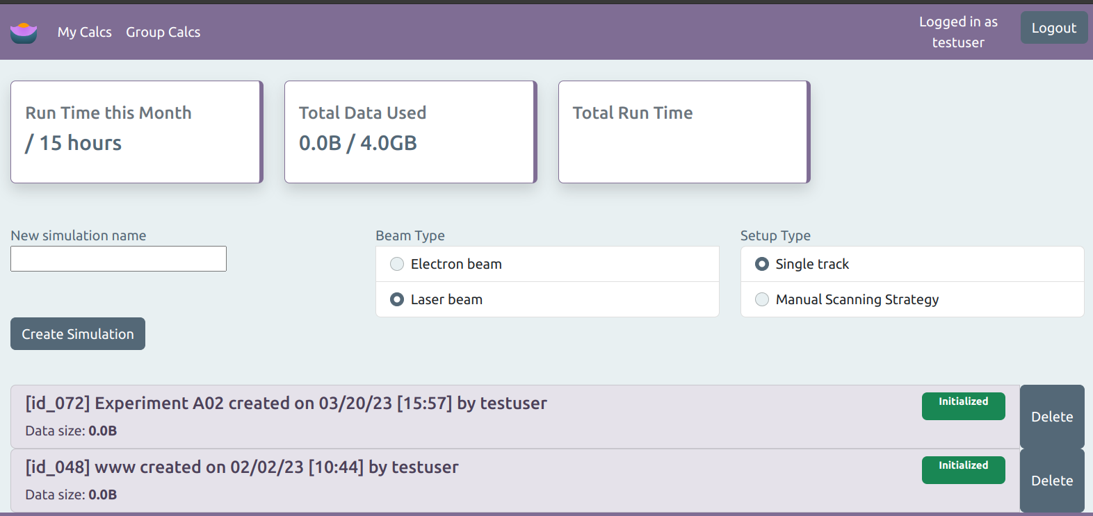
All input data can be filled in the windows:
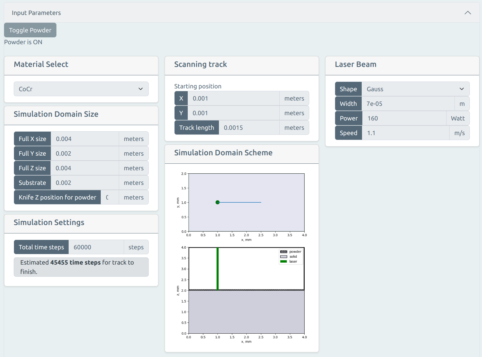
After entering each number, it is automatically recorded in the input file, and the calculation domain scheme in the Simulation Domain Scheme window is updated.
A JSON file is generated below. It can be used as a template for the input in the full KiSSAM version. The syntax is explained here
Powder Generation
To add a powder layer, click the Toggle Powder button. The simulation domain scheme will be automatically generated in the Simulation Domain Scheme window.
Attention
Make sure that the upper edge of the powder layer is below the top edge of the simulation domain (substrate + powder thickness < Full Z size) and above the top edge of the substrate!
The generation of the powder layer is performed by a separate software module. Therefore, when adding a powder layer, the calculation time will increase by several minutes (depending on the layer thickness and the size of the simulation domain). We recommend setting the thickness of the powder layer between 30 and 100 μm. In the trial version of the program, it is not possible to modify the particle size distribution of the powder. This can only be done in the full version of the program. In this version, the distribution is fixed in the program’s internal settings. The user can only adjust the thickness of the powder layer.
Calculation Run
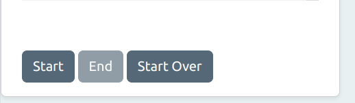
Once all the parameters are defined, an input file is automatically generated. To start the calculation, click the Start button.
Calculation status will be displayed below the Progress label. The calculation itself will start when resources are allocated on the remote machine. This process may take a few minutes. The current status is indicated in the Virtual Machine (VM) status: line.
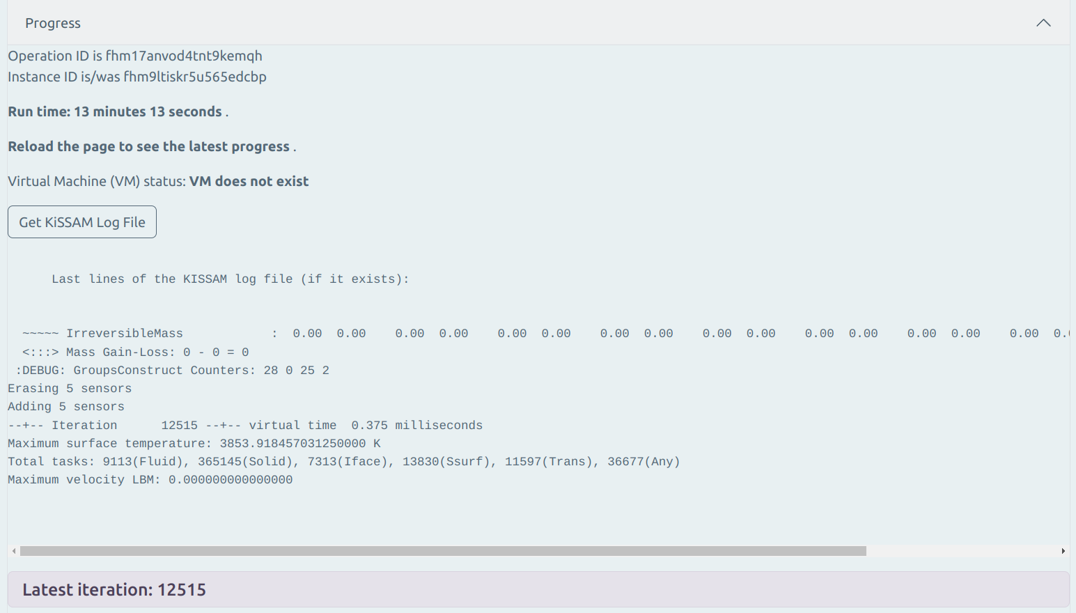
Below the status line, the current part of the KiSSAM log file is displayed. The full file can be accessed by clicking the ‘Get KiSSAM Log File’ button once the process is running. Please refresh your browser page to see the changes.
Hint
Web interface requests the simulation progress data and simulation output only when the page is resfreshed
Hint
Whenever anything is not clear about the simulation progress and output, refresh the web page.
Restarting the Calculation
If you want to stop the current calculation and restart it with modified parameters, click End and then click Start Over. The current calculation will be stopped, and the parameters you have set will be saved in the interface. You can modify one or more parameters and start the calculation again (under the same name and ID) by clicking the Start button. If the Start button is inactive, please wait and refresh your browser page.
Simulation Results
Only a portion of the complete simulation results are obtainable in the trial version. Simulation results are available for inspection in the progress of the calculation. There is no need to wait for the process to complete to view the current results. Once the initial output files have been generated (which takes about 10 minutes), you can view the results in the ‘Output’ section. If you can’t see the output data or want to refresh the displayed data, please refresh your browser page.
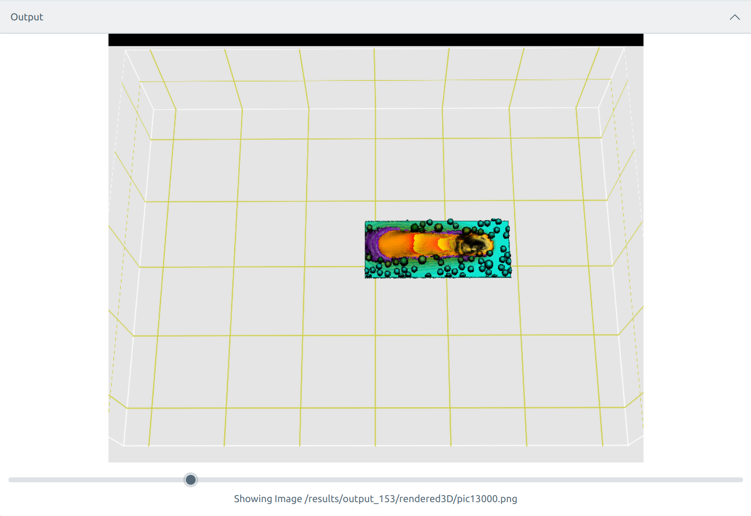
1. Volumetric Image of the meltpool
This allows you to monitor the dynamics of the meltpool during the melting process. The generated image is saved every 1000 time steps (at a step of 30 ns it corresponds to 30 microseconds of real time). You can navigate through the frames of the image using the slider below the image or, after clicking on the slider once, with the keyboard arrow keys (→, ←). The iteration number is indicated in the image caption and in the name of the PNG file.
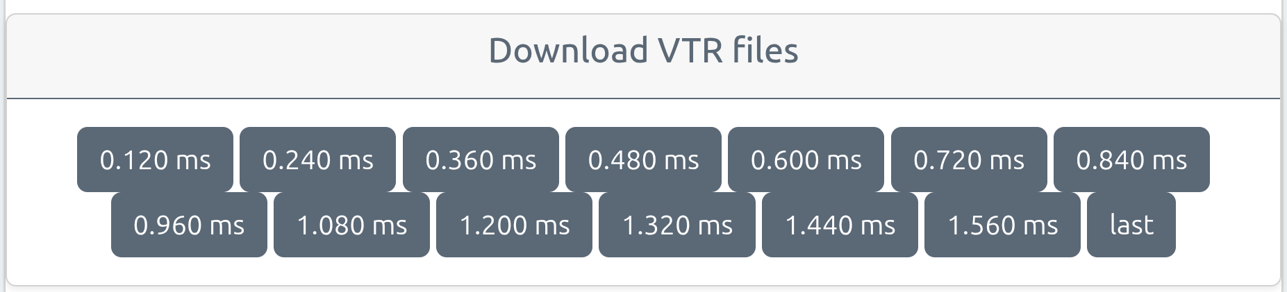
2. Temperature, Velocity and Geometry
Each 4000 time steps and after the simulation is finished the mesh is saved into VTR files, which can be opened with third party software such as Paraview. Download the files by clicking on the buttons.
3. Track Parameters:
Depth, height, and width profiles of the track along the scanning direction will be automatically generated when you click the Get Track Parameters button.

The graphs can be scrolled by clicking on the >, < symbols. The graphs show the height profile of the track at the center cross-section, the depth of melting at the center cross-section, the maximum height of the track, the maximum depth of melting, the maximum width of the track, and the width at the substrate level.
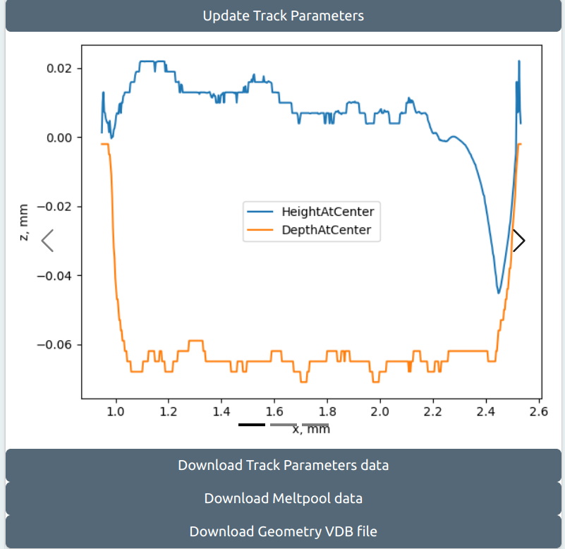
The data can be downloaded as a text file by clicking the Download Track Parameters Data button.
4. Meltpool Parameters
Meltpool Parameters can be downloaded as a text file by clicking the ‘Download Meltpool Data’ button. MeltpoolStats.dat is a text file containing time-dependent depth, height, and width of the
meltpool.
5. Solidified Geometry
Volumetric data in VDB format can be downloaded by clicking the ‘Download Geometry VDB file’ button. This file can be processed or visualized using third-party free applications such as In vdb_view or Blender.
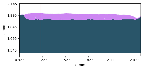
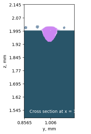
6. Cross-sections
Cross-sections of the track can be generated by specifying the X coordinate (along the laser or electron beam scanning direction). Clicking the ‘Get X Cross Sections’ button generates an image displaying cross-sectional profiles of the track along the scanning axis and a transverse section at the user-specified X coordinate. The value in the coordinate input box is automatically reset to the default value. The melted region is shown in magenta, while the dark region represents the substrate.
Completion of the calculation
The calculation can be stopped by clicking the End button on the simulation page or the Delete button in the list of user simulations. The calculation ends automatically when one of the following conditions is met:
The calculation of the total number of time steps specified in the Total time steps window
- has completed
Time quota for a single calculation (1.5 hours) is exceeded
Total memory quota (10 GB) has exceeded
Total calculation time quota per month (9 hours) is exceeded
The simulation is terminated due to an error.