Sensors¶

Introduction¶

KiSSAM can simulate the readings for the two type of detectors: radiation detectors to measure emitted and reflected electromagnetics waves, as well as detectors of back-scattered electrons.

General setup¶

The Sensors section can contain the two fields: Default and Array.

Default is a default setting for every sensor that is added to the simulation.

Array is an array. For every element of an array, a sensor is added to the simulation. Every element should be represented by JSON data with the same fields that are present in the default sensor. If any field is not specified, the default value is taken.

If the sensor readings are not required, an empty array should be specified to save the computational cost.

Backscattered Electrons¶

In KiSSAM, each simulated electron from the source are traced inside the material, reducing its kinetic energy along the path. Both elastic and inelastic scattering processes are taken into account. In the Monte-Carlo model, the electron trajectory in the material is approximated by a series of straight line segments with a randomly chosen length. The energy loss is modelled by reducing the electron energy at each line segment between two collisions. In the scattering events, the energy is deposited as a volume heat source at the corresponding cells for the LBM temperature model. The electrons can be fully absorbed in the material, if all energy is deposited, or leave the material otherwise.

The electrons that leave the material can be measured by the detectors.

Obviously, the number of the model electrons is small relative to the number of real electron. By default, one electron ray falls on each cell on the surface, which proves to be enough for accurate energy deposition. The parameter can, and should be increased for simulating backscattered electron voltage.

Warning

For low noise in the detector measurements, increase the Beam.RaysPerCell parameter. The defaul value is too low. Set it to a perfect square number, such as 100.

Input¶

To measure backscattered electron voltage, set the deterctor type to Electrons.

The two other fields are relevant for the detector setting: Origin and Size.

Origin are the three coordinates of the detector, which are specified in meters relative to the origin of the simulation domain.

Note

The detection works outside the simulation domain. The coordinates of the origin should be outside the simulation area, specified in sizes.FullXapprox, sizes.FullYapprox, sizes.FullZapprox

The electrons which approach the origin closer than Size/2 (meters) are counted by the detector.

Size can take a special value -1. A detector with Size equal to -1 will count all electrons which are not absorbed by the solid or liquid material.

Here is an example:

 "Sensors":{
    "Default":{
       "DetectType":"Electrons",
       "Size":0.05
    },
    "Array":[
       { "Origin":[ 0.006, 0.006, 0.3006 ]},
       { "Origin":[ 0.2302, 0.006, 0.1933 ]},
       { "Origin":[ 0.2902, 0.006, 0.0782 ]},
       { "Size":-1, "Origin":[ 0, 0, 0 ] }
    ]
 },
 "sizes":{
    "FullZapprox":0.001,
    "FullYapprox":0.0012,
    "FullXapprox":0.0012,
    "substrate":0.0006
    },
"ScanStrategy": {
  "Beam": {
    "type"     : "Ebeam",
    "SuppressBackScattering": 0,
    "RaysPerCell": 100
    }
 }

Here, all sensors detect backscattered electrons. The first sensor is directly above the center of the simulation area, 30 cm above the surface. The next two sensors measure electrons scattered at an angle. The size of the first three sensors is 5 cm. This means, that any electron that enters a sphere (5 cm in diameter) located at the origin coordinates, is counted.

The size of the last sensor is -1. It will count every electron that leaves the material.

Output¶

When the sensors exist in a simulation, the sensors.dat file in the output directory is not empty. It contains a table. Each column represents a sensor from the Sensors.Array. Each row is the reading of the sensor: the power (W) measured during the config.IterationSubstepsRate time steps, multiplied by the value of config.IterationSubstepsRate.

In the example above, the file will contain four columns.

Infrared Camera Simulation¶

Radiation sensors (photo-detectors) can be specified to collect emission from the melted and solid area.

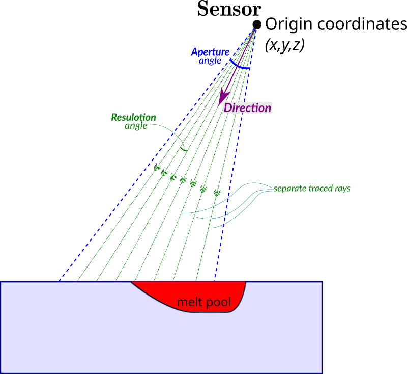
Each sensor is a point with coordinates \((x,y,z)\) (origin), Direction vector, Aperture view angle, Resolution angle between individual rays traced from the origin point inside the cone and Wavelength band response. Each separate ray inside the sensor’s cone is traced until the collision point with the meltpool or solid surface and the emission power of this point is calculated from temperature in accordance with Plank’s law and collected by the sensor.

So the sensors signal is calculated at every time step with the following formula:

\[\text{Emission energy [J]} = \sum\limits_{i} \Delta t \varepsilon \cfrac{\pi {|\vec r_i|}^{ 2}\beta^2}{4} \int\limits_{\lambda_1}^{\lambda_2}\cfrac{2hc^2}{\lambda^5 \left(e^{\frac{hc}{\lambda k_B T_i}}-1\right)}d\lambda,\]

where \(\Delta t\) is time step, \(\vec r_i=\vec p_i-\vec s_i\) is a ray vector pointed from the sensor’s origin point, \(\vec s_i\) to the ray’s intersection point with the surface \(\vec p_i\), \(T_i\) is the surface temperature of the point \(\vec p_i\), \(\beta\) is the sensor’s resolution angle, \(h\), \(c\), \(k_B\) are Plank’s constant, light speed and Boltzmann constant, and \([\lambda_1,\lambda_2]\) is the wavelength band of the sensor’s response. Emissivity constant \(\varepsilon\) is assumed to be 1 now. The sum \(\sum\limits_i\) is accumulated over the full set of the rays back-traced from the sensor as shown in the figure above.

Input¶

Below is the example input for photodetector sensor array. Here we reproduce the measurement from

[sensors]

Heigel, Jarred C., and Brandon M. Lane. “Measurement of the melt pool length during single scan tracks in a commercial laser powder bed fusion process.” Journal of Manufacturing Science and Engineering 140, no. 5 (2018): 051012

The setup is PBF-L with In625 flat substrate, the laser beam width is \(D_{4\sigma}=100\) microns, the laser speed is 0.2 m/s, and the laser power is 49 W.

{
 "ScanStrategy": {
     "Beam": {
         "Speed": 0.2,
         "Power": 49.0,
         "Width": 0.0001,
         "type": "Laser"
     },
     "SingleTrack": {
         "length": 0.001,
         "startPosX": 0.0005,
         "startPosY": 0.0005
     },
     "Type": "SingleTrack"
 },
 "Substrate": {
     "initGeometryVDBfile": ""
 },
 "Powder": {
     "initSpheresVDBfile": ""
 },
 "sizes": {
     "substrate": 0.001,
     "FullXapprox": 0.002,
     "FullYapprox": 0.001,
     "FullZapprox": 0.002
 },
 "Visual": {
     "RenderOnlyMeltpool": false,
     "3DrenderedDomainSize": [
         0.002,
         0.001,
         0.0005
     ]
 },
 "Material": "In625",
 "Sensors": {
     "Default": {
         "Aperture": 1.4142135623730953e-05,
         "Resolution": 2.0000000000000003e-06,
         "WavelengthBand": [
             1.35e-06,
             1.6e-06
         ]
     },
     "Array": [
                 {
             "Origin": [
                 0.000245,
                 0.000345,
                 1
             ]
         },
         {
             "Origin": [
                 0.000245,
                 0.000355,
                 1
             ]
         },
         ...
         ]
     }
 }

You can download the input file here.

The sensor type is Radiation by default, so the DetectType field is not specified.

The wavelength band is [1350 nm, 1600 nm] as described in [sensors].

The sensor matrix is prepared according to the image:

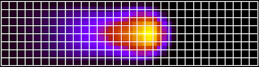
Each sensor aperture is a circumscribed circle over each pixel/square having 10 micron size. There are 151 x 32 sensors in total.

Output¶

When the sensors exist in a simulation, the sensors.dat file in the output directory is not empty. It contains a table. Each column represents a sensor from the Sensors.Array. Each row is the reading of the sensor: the power (W) measured during the config.IterationSubstepsRate time steps, multiplied by the value of config.IterationSubstepsRate.

In the example above, the file will contain 151x32=4832 columns.

787081e-22  2.787081e-22  2.787081e-22  2.787081e-22  2.787081e-22  2.787081e-22  ...  2.787078e-22  2.787078e-22  2.787078e-22  2.787078e-22  2.787078e-22  2.787078e-22
787075e-22  2.787075e-22  2.787075e-22  2.787075e-22  2.787075e-22  2.787075e-22  ...  2.787075e-22  2.787075e-22  2.787075e-22  2.787075e-22  2.787075e-22  2.787075e-22
787075e-22  2.787075e-22  2.787075e-22  2.787075e-22  2.787075e-22  2.787075e-22  ...  2.787075e-22  2.787075e-22  2.787075e-22  2.787075e-22  2.787075e-22  2.787075e-22
787075e-22  2.787075e-22  2.787075e-22  2.787075e-22  2.787075e-22  2.787075e-22  ...  2.787075e-22  2.787075e-22  2.787075e-22  2.787075e-22  2.787075e-22  2.787075e-22
787075e-22  2.787075e-22  2.787075e-22  2.787075e-22  2.787075e-22  2.787075e-22  ...  2.787075e-22  2.787075e-22  2.787075e-22  2.787075e-22  2.787075e-22  2.787075e-22
         ...           ...           ...           ...           ...           ...  ...           ...           ...           ...           ...           ...           ...
723407e-21  1.955601e-21  2.208074e-21  2.483935e-21  2.777268e-21  3.083244e-21  ...  2.787075e-22  2.787075e-22  2.787075e-22  2.787075e-22  2.787075e-22  2.787075e-22
704548e-21  1.931576e-21  2.177066e-21  2.446802e-21  2.733296e-21  3.028844e-21  ...  2.787075e-22  2.787075e-22  2.787075e-22  2.787075e-22  2.787075e-22  2.787075e-22
696174e-21  1.906045e-21  2.134429e-21  2.404739e-21  2.687672e-21  2.978568e-21  ...  2.787075e-22  2.787075e-22  2.787075e-22  2.787075e-22  2.787075e-22  2.787075e-22
838532e-21  2.062163e-21  2.307727e-21  2.609537e-21  2.935415e-21  3.268173e-21  ...  2.787075e-22  2.787075e-22  2.787075e-22  2.787075e-22  2.787075e-22  2.787075e-22
953874e-21  2.191602e-21  2.453274e-21  2.777907e-21  3.133159e-21  3.496277e-21  ...  2.787075e-22  2.787075e-22  2.787075e-22  2.787075e-22  2.787075e-22  2.787075e-22

Sensors¶

Introduction¶

General setup¶

Backscattered Electrons¶

Input¶

Output¶

Infrared Camera Simulation¶

Input¶

Output¶

Table of Contents

Previous topic

Next topic

This Page