
QUICKSTART
System Requirements
KiSSAM requires a workstation with Linux OS and at least one NVidia GPU. The minimal hardware requirements are
x86 CPU (Intel i5 processor or AMD Ryzen 5 desktop or server);
NVidia GPU Ampere or newer architecture with more than 16 GB GPU memory;
RAM 32 GB RAM.
Software requirements
Ubuntu 22.04+
CUDA 12.1
nVidia driver 530.xxx.xx
Docker and docker-compose-v2
nvidia-container-toolkit, nvidia-container-runtime
Recommended third party software
A text editor or JSON editor for configuration.
vdb_viewor Blender for viewing output geometry.Preferred data analysis software: Paraview, MS Excel, Matlab, etc.
X server
VirtualGL
OpenVDB
Installation and Setup
Please contact our support team for the setup of the KiSSAM package on your system.
Currently, trial versions are distributed with the Docker containers.
You will need the kissam.tar image and the license file.
Running with Docker
Below is the procedure for running KiSSAM in Docker CLI, from the Linux Terminal.
First, after obtaining the KiSSAM image, you need to load it once into your system. Open the terminal, navigate to the directory, where the kissam.tar file is located, and type
docker load -i kissam.tar
Depending on the docker installation, you may need to run this in sudo mode. If you prefer to disable sudo mode, run
sudo usermod -aG docker $USER
You can immediately try running the code:
docker run --gpus all --rm -v .:/calc -it kissam
Here is the simulation procedure we recommend for the beginners.
First, create a directory for your simulation, and navigate into it
> mkdir my_first_simulation
> cd my_first_simulation
In it, you will need an input JSON file, and a license file.
>  cp  ~/Downloads/license.lic license.lic
>  echo '{"licenseFile": "license.lic"}' > input.json
An empty JSON file corresponds to the default simulation settings. However, the user license file has to be specified.
docker run --gpus all -e USER_ID=$(id -u) -e GROUP_ID=$(id -g) -e INPUT_JSON_FILE=input.json --rm -v .:/calc -it kissam
The options we used here are:
--gpus allto use your GPU device. You can use another option, such as--gpus '"device=1"'
-eare the environment variables. The input JSON file has to be specified.
-v .:/calcthe current directory will be mounted to the/calcdirectory in the container. Therefore, if you need any additional files for the input, they should also be placed in the current directory.
Proceed to Check Output.
To terminate the computation before it is complete, use Ctrl + C in that terminal, or the kill command.
If KiSSAM is installed without container
KiSSAM is run from Linux terminal.
The starting script and default simulation setup file
start_calc.sh
and
default.json
are provided with the distribution.
Open terminal and make calculation directory
> mkdir my_calc
> cd my_calc
Create the input JSON file. The minimal JSON file has to contain the information on the license.
> echo '{"licenseFile": "my-license-file.lic"}' > input.json
Run the simulation startup script with the input file
> INPUT_JSON_FILE=input.json /opt/KiSSAM/start_calc.sh
Simulation is started with the default parameters. The parameters of the simulation are specified in this input JSON file. You can get the examples from User Cases and refer to the JSON specification for the details. Alternatively, you can copy the default JSON file and edit it: change the relevant fields and erase irrelevant fields.
The free GPU will be chosen automatically.
If all GPUs on the computer are busy, it may not start.
You can use --wait option.
It makes the startup script wait until any GPU is released and do not return control in terminal.
> INPUT_JSON_FILE=input.json /opt/KiSSAM/start_calc.sh --wait &>log &
Check Output
To check that the startup is successful, confirm that
no errors are output in the terminal
*.logfiles are generated.computation can be confirmed by the
nvidia-smiterminal command
kissam-log-x.log contains simulation log. x is the incremental file number. It is updated during the simulation.
If the lines of the following type are appearing continuously, the simulation is being successfully executed in the background.
--+-- Iteration 0 --+-- virtual time 0.000 milliseconds
PIDXXXXXX.log (XXXXXX is the process ID of the simulation) is a symbolic link to the kissam-log-x.log.
The simulation will end when the maximal number of steps is reached (can be changed in the JSON file), or can be interrupted with the kill command in terminal.
To end simulation before it is finished
> kill -9 XXXXXX
Expected simulation time is several hours. Check the process during the simulation by looking at the output files.
Output
By default the output result is in the output directory (can be changed in the JSON file).
full_params.jsonrecords all the parameters of the simulation, inluding both user specified and the default parameters, and the KiSSAM version as well.Warning
Even though it is a JSON file, it should never be used for the input of a simulation. Using it as an input file may cause errors that are difficult to track. To prevent such errors, the JSON syntax in it is broken on purpose.
init_geometry.vdbis the initial geometry (powder+substrate) of the powder bed. OpenVDB is a library and file format for the interoperability and storage of volumetric data, and it is supported by various 3D software. The file contains two grids with the following names:FillingFrac, typefloat, is the filling fraction of mesh cells;ParticleIds, typeInt32, are identifiers which help to distinguish types of solid: powder particles, substrate, melted material.
Note that the cells are not activated in this output, so third party software may not render it.
A script to activate the cells for visualization is provided with the software.
The file metadata includes all input parameters of the simulation.
* geometry.vdb is the latest geometry computed in the simulation.
The file also contains both FillingFrac and ParticleIds grids plus full metadata.
If the geometry was written while the simulation is in progress and melt is not solidified yet, the grids named Temperature and Velocity represent corresponding parameters in the melt pool region.
Note that here the temperature is written only on the meltpool region. The temperature in the whole simulation region is written in the VTK file Temp.vtk.
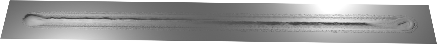
Fig. 1 Example of the vdb file loaded and rendered in Blender. Surface of a single track on a bare substrate
rendered3D/is a directory with rendered 3D views of the simulation.
Only a part of the grid, centered around the laser incidence point, is shown. The visualization box moves with the laser. The size of visualized area can bet changed in the JSON file. The rendered image inside the box shows only the Meltpool~Grid: a domain for fluid dynamics simulation of adaptive size that contains the meltpool.
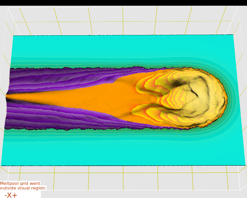
Fig. 2 Example of the rendered 3D image in the output
cross-sections/is a directory with PNG images with 2D cross-sections of meltpool grid in different positions.
It contains subdirectories with names X*****, which contain cross sections at \(x=\)***** (in μm) and Y*****, which contain cross sections at \(y=\)*****.
The images inside are named sec-itt.png: the cross sections in the specified position at times \(t=\)t.
The meltpool grid is adaptive, therefore, cross-section images have different sizes, and may be empty if the section does not intersect the meltpool grid at the moment. KiSSAM includes utility scripts that combine the images and pad them so that sizes match and generate informative animations.

Fig. 3 Example of cross-section in the output. Yellow grid lines show 100 μm scale.
Use the pad_images.sh script to pad images.
palletes_raw.png,palettes_crop.png– images of color maps used for visualizations.
Three separated color scales are used for liquid, for solidified material and for solid that was not melted. The temperature range is from 0K to 3000K. The palette depends on the material properties, namely, melting and solidification temperatures.

|

Fig. 4 Colormap images output in the code¶ |
entalpy_diagnostics.log– logfile for material temperature-dependent enthalpy. This log is used to verify correct usage of theMaterial.HeatCapacityVolValsandMaterial.HeatCapacityRefTempparameters.Temp.vtk— the binary VTK.vtrfiles (VTK rectilinear grid) with global temperature distribution and tractile grid cell fractions.outTprobes.dat– text files with temperature in probes with coordinates specified in input filemyTprobes.dat.
The file contains a table with a column for each probe and a row for each time iteration. The first column is an iteration number.
meltpoolStats.dat— text file with time-dependent meltpool depth, height and width.
To get these dimensions, the fluid cells with maximal/minimal \(x\), \(y\), and \(z\) coordinates are found, as well as maximal/minimal \(x\), \(y\) at the level of substrate. From these values, the meltpool dimensions are estimated.
absorbedEnergy.dat— time-dependent absorbed energy by solid and liquid phases.
What’s next
Refer to the user cases provided with the software. We recommend to run the user cases to get more experience with KiSSAM usage.