Beam Acceleration

Introduction

Numerical simulation gives us full control of the energy source power, shape, and position. In one simulation, by gradually accelerating the beam, we can observe how the melting regime changes.

Setup

In the simulation, an accelerating laser beam melts an In625 powder layer on a flat substrate. The beam width is 100 μm, the beam power is 200 W.

The accelerating beam is with the manual scan path in the JSON input file. With an external software, we generated the following file:

0.0 0.0005 0.0005
1e-08 0.0005000000000006661 0.0005
2e-08 0.0005000000000026645 0.0005
3.0000000000000004e-08 0.0005000000000059997 0.0005
4e-08 0.000500000000010667 0.0005
5e-08 0.0005000000000166667 0.0005
6.000000000000001e-08 0.0005000000000239986 0.0005
7e-08 0.0005000000000326672 0.0005
8e-08 0.0005000000000426637 0.0005
9e-08 0.0005000000000540013 0.0005
1e-07 0.0005000000000666667 0.0005
...

The first column here is time (s), the second and the third are the beam positions in x and y (m). The laser starts at \(x=0.5\) mm, \(y=0.5\) mm in the \(12\text{cm} \times 1\text{mm} \times 6\text{mm}\) domain. The y coordinate is constant. The x coordinate changes as shown in the figure:

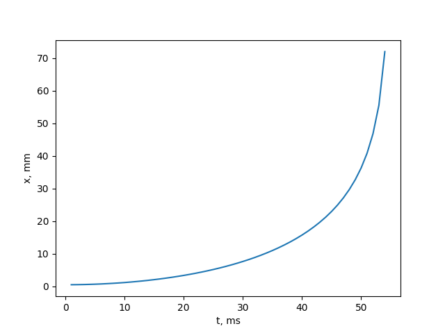
Fig. 76 x position vs time in the input data

In the input JSON file, we set the filename in the ScanStrategy.XYpositions field, and set the scanning strategy type to XYpositions:

"ScanStrategy": {
    ...
    "Type": "XYpositions",
    "XYpositions":"xy.dat"
    }

Results

We see the change in the meltpool width and depth, as well as qualitative change in the process. At the beginning, a deep keyhole is observed. The melt regime changes to a stable melt, and deteriorated into balling with the increase in the beam speed.

Please click on the image below to view the animation of the simulation results.

Fig. 77 Click on the image to view the video